Regression. Such a strange name to be applied to our good friend, the method of least-squares curve fitting. How did that happen?
My dictionary says that regression is the act of falling back to an earlier state. In psychiatry, regression refers to a defense mechanism where you regress – fall back – to a younger age to avoid dealing with the problems that us adults have to deal with. Boy, can I relate to that!

Then there’s regression therapy, and regression testing…

All statisticians recognize the need for regression
Then there’s regression therapy, and regression testing…
Changing the subject radically, the “method of least squares” is used to find the line or curve that "best" goes through a set of points. You look at the deviations from a curve – each of the individual errors in fitting the curve to the points. Each of these deviations is squared and then they are all added up. The least squares part comes in because you adjust the curve so as to minimize this sum. When you find the parameters of the curve that give you the smallest sum, you have the least squares fit of the curve to your data.
For some silly reason, the method of least squares is also known as regression. It is perhaps an interesting story. I have been in negotiations with Random House on a picture book version of this for pre-schoolers, but I will give a preview here.
Prelude to regression
Let’s scroll back to the year 1766. Johann Titius has just published a book that gave a fairly simple formula that approximated the distances from the Sun to all the planets. Titius had discovered that if you subtract a constant from the size of the each orbit, the planets all fell in a geometric progression. After subtracting a constant, each planet was twice as far from the Sun as the one previous. Since Titius discovered this formula, it became known as Bode’s law.
I digress in this blog about regressing. Stigler’s law of eponymy says that all scientific discoveries are named after someone other than the original discoverer. Johann Titius stated his law in 1766. Johann Bode repeated the rule in 1772, and in a later edition, attributed it to Titius. Thus, it is commonly known as Bode’s law. Every once in a while it is called as the Titius-Bode law.
I digress in this blog about regressing. Stigler’s law of eponymy says that all scientific discoveries are named after someone other than the original discoverer. Johann Titius stated his law in 1766. Johann Bode repeated the rule in 1772, and in a later edition, attributed it to Titius. Thus, it is commonly known as Bode’s law. Every once in a while it is called as the Titius-Bode law.
The law held true for six planets: Mercury, Venus, Earth, Mars, Jupiter, and Saturn. This was interesting, but didn’t raise many eyebrows. But when Uranus was discovered in 1781, and it fit the law, people were starting to think seriously about Bode’s law. It was more than a curiosity; it was starting to look like a fact.
But there was just one thing I left out about Bode’s law – the gap between Mars and Jupiter. Bode’s law worked fabulous if you pretended there was a mysterious planet between these two. Mars is planet four and we will pretend that Jupiter is planet six. Does planet five exist?


Now where did I put that fifth planet???
Scroll ahead to 1800. Twenty four of the world’s finest astronomers were recruited to go find the elusive fifth planet. On New Year’s Day of 1801, the first day of the new century, a fellow by the name of Giuseppe Piazzi discovered Ceres. Since it was moving with respect to the background of stars, he knew it was not a star, but rather something that resided in our the solar system. At first Piazzi thought it was a comet, but he also realized that it could be the much sought after fifth planet.
How could he decide? He needed to have enough observations over a long enough time period of time so that the orbital parameters of Ceres could be determined. Piazza observed Ceres a total of 24 times between January 1 and February 11. Then he fell ill, suspending his observations. Now, bear in mind that divining an orbit is a tricky business. This is a rather short period of time from which to determine the orbit.
It was not until September of 1801 that word got out about this potential planet. Unfortunately, Ceres had slipped behind the Sun by then, so other astronomers could not track it. The best guess at the time was that it should again be visible by the end of the year, but it was hard to predict just where the little bugger might show his face again.
Invention of least squares curve fitting
Invention of least squares curve fitting
Enter Karl Friedrich Gauss. Many folks who work with statistics will recall his name in association with the Gaussian distribution (also known as the normal curve and the bell curve). People who are keen on linear algebra will no doubt recall the algorithm called “Gaussian elimination”, which is use to solve systems of linear equations. Physicists are not doubt aware of the unit of measurement of the strength of a magnetic field that was named after Gauss. Wikipedia currently lists 54 things that were named after Gauss.
More digressing...As is the case of every mathematical discovery, the Gaussian distributions was named after the wrong person.The curve was discovered by De Moivre. Did I mention Stigler? Oh... while I am at it, I should mention that Gaussian elimination was developed in China when young Gauss was only -1,600 years old.. Isaac Newton independently developed the idea about 1670. Gauss improved the notation in 1810, and thus the algorithm was named after him.
Back to the story. Gauss had developed the idea of least squares in 1795, but did not publish it at the time. He immediately saw that the Ceres problem was an application for this tool. He used least squares to fit a curve to the existing data in order to ascertain the parameters of the orbit. Then he used those parameters to predict where Ceres would be when it popped its head out from behind the Sun. Sure enough, on New Year’s eve of 1801, Ceres was found pretty darn close to where Gauss had said it would be. I remember hearing a lot of champagne corks popping at the Gaussian household that night! Truth be told, I don't recall much else!


From Gauss' 1809 paper "Theory of the Combination of Observations Least Subject to Error"
The story of Ceres had a happy ending, but the story of least squares got a bit icky. Gauss did not publish his method of least squares until 1809. This was four years after Adrien Marie Legendre’s introduction of this same method. When Legendre found out about Gauss’ claim of priority on Twitter, he unfriended him on FaceBook. It's sad to see legendary historical figures fight, but I don't really blame him.
In the next ten years, the incredibly useful technique of regression became a standard tool in many scientific studies - enough so that it became a topic in text books.
In the next ten years, the incredibly useful technique of regression became a standard tool in many scientific studies - enough so that it became a topic in text books.
Regression
So, that’s where the method of least squares came from. But why do we call it regression?
I’m going to sound (for the moment) like I am changing the subject. I’m not really, so bear with me. It’s not like that one other blog post where I started talking about something completely irrelevant. My shrink says I need to work on staying focused. His socks usually don't match.
Let’s just say that there is a couple, call them Norm and Cheryl (not their real names). Let’s just say that Norm is a pretty tall guy, say, 6’ 5” (not his real height). Let’s say that Cheryl is also pretty tall, say, 6’ 2” (again, not her real height). How tall do we expect their kids to be?
I think most people would say that the kids are likely to be a bit taller than the parents, since both parents are tall – they get a double helping of whatever genes there are that make people tall, right?
One would think the kids would be taller, but statistics show this is generally not the case. Sir Francis Galton discovered this around 1877 and called it “regression to the mean”. Offspring of parents with extreme characteristics will tend to regress (move back) toward the average.
Why would this happen?
As with most all biometrics (biological measurements), there are two components that drive a person’s height – nature and nurture, genetics and environment. I apologize in advance to the mathaphobes who read this blog, but I am going to put this in equation form.
Actual Height = Genetic height + Some random stuff
Here comes the key point: If someone is above average in height, then it is likely that the contribution of “some random stuff” is a bit more than average. It doesn’t have to be, of course. Someone can still be really tall and still shorter than genetics would generally dictate. But, if someone is really tall, it’s likely that they got two scoops: genetics and random stuff.
So, what about the offspring of really tall people? If both parents are really tall, then you would expect the genetic height of the offspring to be about the same as that of the parents, or maybe a bit taller. But (here comes the second part of the key point) if both parents were dealt a good hand of random stuff, and the hand of random stuff that the children are dealt is average, then it is likely that the offspring will not get as good a hand as the parents.
The end result is that the height of the children is a balance between the upward push of genetics and the downward push of random stuff. In the long run, the random stuff has a slight edge. We find that the children of particularly tall parents will regress to the mean.

The end result is that the height of the children is a balance between the upward push of genetics and the downward push of random stuff. In the long run, the random stuff has a slight edge. We find that the children of particularly tall parents will regress to the mean.
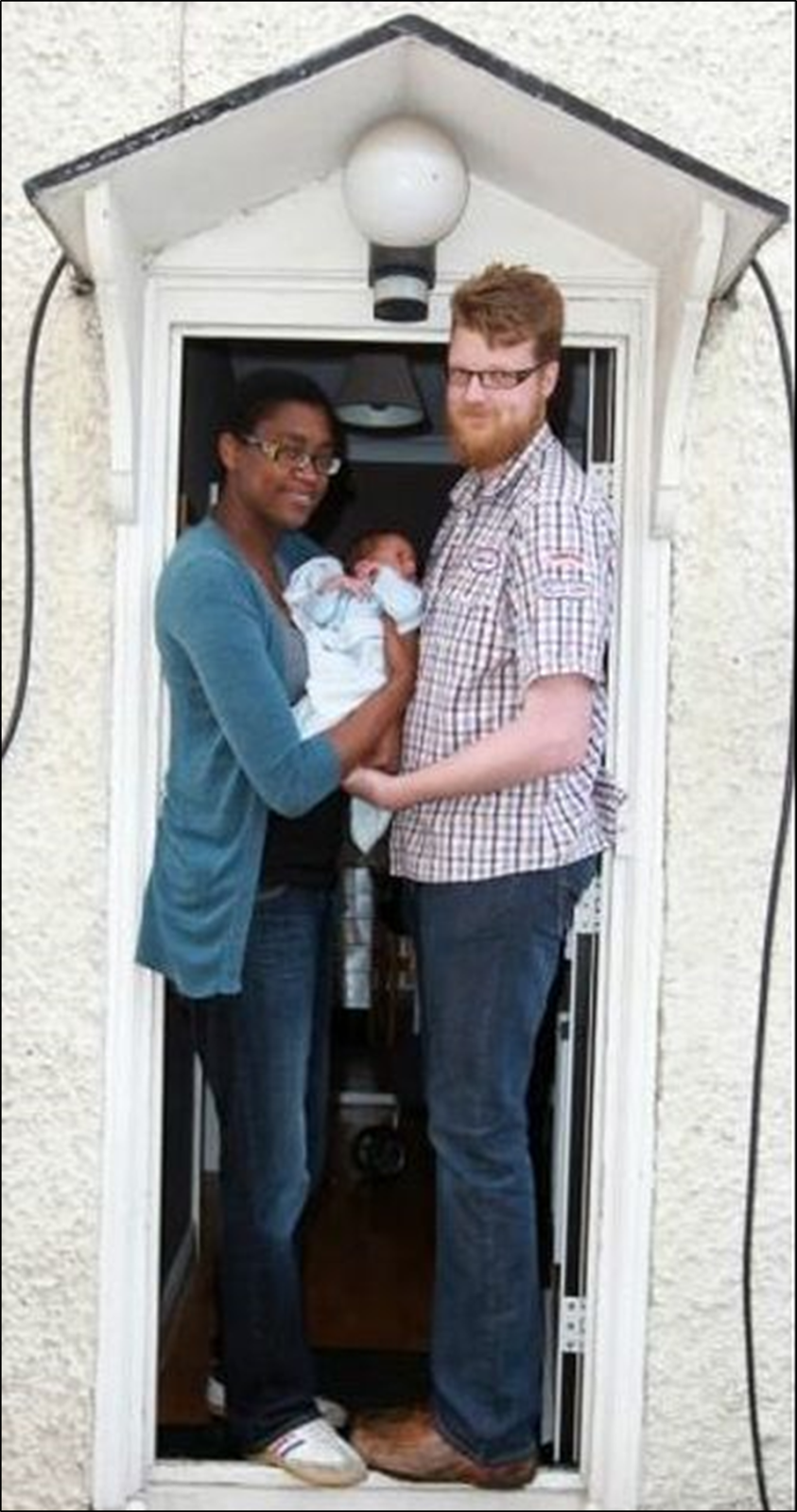
We expect the little shaver to grow up to be a bit shorter than mom and pop
Galton and the idea of "regression towards mediocrity"
Francis Galton noticed this regression to the mean when he was investigating the heritability of traits, as first described in his 1877 paper Typical Laws of Heredity. He started doing all kinds of graphs and plots and stuff, and chasing his slide rule after bunches of stuff. He later published graphs like the one below, showing the distribution of the heights of adult offspring as a function of the mean height of their parents.
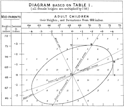
Francis Galton noticed this regression to the mean when he was investigating the heritability of traits, as first described in his 1877 paper Typical Laws of Heredity. He started doing all kinds of graphs and plots and stuff, and chasing his slide rule after bunches of stuff. He later published graphs like the one below, showing the distribution of the heights of adult offspring as a function of the mean height of their parents.

From Galton's paper "Regression towards mediocrity in hereditary stature", 1886
(For purposes of historical accuracy, Galton's 1877 paper used the word revert. The 1886 paper used the word regression.)
In case you're wondering, this is what we would call a two-dimensional histogram. Galton's chart above is a summary of 930 people and their parents. You may have to zoom in to see this, but there are a whole bunch of numbers arranged in seven rows and ten columns. The rows indicate the average height of the parent, and the columns are the height of the child. Galton laid these numbers out on a sheet of paper (like cells in a spreadsheet) and had the clever idea of drawing a curve that traced through cells with similar values. He called these curves isograms, but the name didn't stick. Today, they might be called contour lines; on a topographic plot, they are called isoclines, and on weather maps, we find isobars and isotherms.
Galton noted that the isograms on his plot of heights were a set of concentric ellipses, one of which is shown in the plot above. The ellipses were all tilted upward on the right side.
As an aside, Galton's isograms were the first instance of ellipsification that I have seen. Coincidentally, the last blog post that I wrote was on the use of ellipsification for SPC of color data. I was not aware of Galton's ellipsification when I started writing this blog post. Another example of the fundamental inter-connectedness of all things. Or an example of people finding patterns in everything!
Galton did not give a name to the major axis of the ellipse. He did speak about the "mean regression in stature of a population", which is the tilt of the major axis of the ellipse. From this analysis, he determined that number to be 2/3, which is to say, if the parents are three inches taller than average, then we can expect (on average) that the children be two inches above average.
So, Galton introduced the word regression into the field of statistics of two variables. He never used it to describe a technique for fitting a line to a set of data points. In fact, the math he used to derive his mean regression in stature bears no similarity to the linear regression by least squares that is taught in stats class. Apparently, he was unaware of the method of least squares.
Enter George Udny Yule
George Udny Yule was the first person to misappropriate the word regression to mean something not related to "returning to an earlier state". In 1897, he published a paper called On the Theory of Correlation in the Journal of the Royal Statistical Society. In this paper, he borrowed the concepts implied by the drawings from Galton's 1886 paper, and seized upon the word regression. In his own words (p. 177), "[data points] range themselves more or less closely round a smooth curve, which we shall name the curve of regression of x on y." In a footnote, he mentions the paper by Galton and the meaning that Galton had originally assigned to the word.
In the rest of the paper, Yule lays out the equations for performing a least squares fit. He does not claim authorship of this idea. He references a textbook entitled Method of Least Squares (Mansfield Merriman, 1894). Merriman's book was very influential in the hard sciences, having been first published in 1877, with the eighth version in 1910.
So Yule is the guy who is responsible for bringing Gauss' method of least squares into the social sciences, and in calling it by the wrong name.
Yule reiterates his word choice in the book Introduction to the Theory of Statistics, first published in 1910, with the 14th edition published in 1965. He says: In general, however, the idea of "stepping back" or "regression" towards a more or less stationary mean is quite inapplicable ... the term "coefficient of regression" should be regarded simply as a convenient name for the coefficients b1 and b2.
So. There's the answer. Yule is the guy who gave the word regression a completely different meaning. How did his word, regression, become so commonplace, when "least squares" was a perfectly apt word that had already established itself in the hard sciences? I can't know for sure.

Addendum
Galton is to be appreciated for his development of the concept of correlation, but before we applaud him for his virtue, we need to understand why he spent much of his life measuring various attributes of people, and inventing the science of statistics to make sense of those measurements.
Galton was a second cousin of Charles Darwin, and was taken with the idea of evolution. Regression wasn't the only word he invented. He also coined the word eugenics, and defines it thus:
"We greatly want a brief word to express the science of improving stock, which is by no means confined to questions of judicious mating, but which, especially in the case of man, takes cognisance of all influences that tend in however remote a degree to give to the more suitable races or strains of blood a better chance of prevailing speedily over the less suitable than they otherwise would have had. The word eugenics would sufficiently express the idea..."
Francis Galton, Inquiries into Human Faculty and its Development, 1883, page 17
The book can be summarized as a passionate plea for the need of more research to identify and quantify those traits in humans that are good versus those which are bad. But what should be done about traits that are deemed bad? Here is what he says:
"There exists a sentiment, for the most part quite unreasonable, against the gradual extinction of an inferior race. It rests on some confusion between the race and the individual, as if the destruction of a race was equivalent to the destruction of a large number of men. It is nothing of the kind when the process of extinction works silently and slowly through the earlier marriage of members of the superior race, through their greater vitality under equal stress, through their better chances of getting a livelihood, or through their prepotency in mixed marriages."
Ibid, pps 200 - 201
As an aside, Galton's isograms were the first instance of ellipsification that I have seen. Coincidentally, the last blog post that I wrote was on the use of ellipsification for SPC of color data. I was not aware of Galton's ellipsification when I started writing this blog post. Another example of the fundamental inter-connectedness of all things. Or an example of people finding patterns in everything!
Galton did not give a name to the major axis of the ellipse. He did speak about the "mean regression in stature of a population", which is the tilt of the major axis of the ellipse. From this analysis, he determined that number to be 2/3, which is to say, if the parents are three inches taller than average, then we can expect (on average) that the children be two inches above average.
So, Galton introduced the word regression into the field of statistics of two variables. He never used it to describe a technique for fitting a line to a set of data points. In fact, the math he used to derive his mean regression in stature bears no similarity to the linear regression by least squares that is taught in stats class. Apparently, he was unaware of the method of least squares.
Enter George Udny Yule
George Udny Yule was the first person to misappropriate the word regression to mean something not related to "returning to an earlier state". In 1897, he published a paper called On the Theory of Correlation in the Journal of the Royal Statistical Society. In this paper, he borrowed the concepts implied by the drawings from Galton's 1886 paper, and seized upon the word regression. In his own words (p. 177), "[data points] range themselves more or less closely round a smooth curve, which we shall name the curve of regression of x on y." In a footnote, he mentions the paper by Galton and the meaning that Galton had originally assigned to the word.
In the rest of the paper, Yule lays out the equations for performing a least squares fit. He does not claim authorship of this idea. He references a textbook entitled Method of Least Squares (Mansfield Merriman, 1894). Merriman's book was very influential in the hard sciences, having been first published in 1877, with the eighth version in 1910.
So Yule is the guy who is responsible for bringing Gauss' method of least squares into the social sciences, and in calling it by the wrong name.
Yule reiterates his word choice in the book Introduction to the Theory of Statistics, first published in 1910, with the 14th edition published in 1965. He says: In general, however, the idea of "stepping back" or "regression" towards a more or less stationary mean is quite inapplicable ... the term "coefficient of regression" should be regarded simply as a convenient name for the coefficients b1 and b2.
So. There's the answer. Yule is the guy who gave the word regression a completely different meaning. How did his word, regression, become so commonplace, when "least squares" was a perfectly apt word that had already established itself in the hard sciences? I can't know for sure.

The word regression is a popular word on my bookshelf
Addendum
Galton is to be appreciated for his development of the concept of correlation, but before we applaud him for his virtue, we need to understand why he spent much of his life measuring various attributes of people, and inventing the science of statistics to make sense of those measurements.
Galton was a second cousin of Charles Darwin, and was taken with the idea of evolution. Regression wasn't the only word he invented. He also coined the word eugenics, and defines it thus:
"We greatly want a brief word to express the science of improving stock, which is by no means confined to questions of judicious mating, but which, especially in the case of man, takes cognisance of all influences that tend in however remote a degree to give to the more suitable races or strains of blood a better chance of prevailing speedily over the less suitable than they otherwise would have had. The word eugenics would sufficiently express the idea..."
Francis Galton, Inquiries into Human Faculty and its Development, 1883, page 17
The book can be summarized as a passionate plea for the need of more research to identify and quantify those traits in humans that are good versus those which are bad. But what should be done about traits that are deemed bad? Here is what he says:
"There exists a sentiment, for the most part quite unreasonable, against the gradual extinction of an inferior race. It rests on some confusion between the race and the individual, as if the destruction of a race was equivalent to the destruction of a large number of men. It is nothing of the kind when the process of extinction works silently and slowly through the earlier marriage of members of the superior race, through their greater vitality under equal stress, through their better chances of getting a livelihood, or through their prepotency in mixed marriages."
Ibid, pps 200 - 201
It seems that Galton favors a kindler, gentler form of ethnic cleansing. I sincerely hope that all my readers are as disgusted by these words as I am.
This blog post was edited on Dec 28, 2017 to provide links to the works by Galton and Yule.
This blog post was edited on Dec 28, 2017 to provide links to the works by Galton and Yule.


