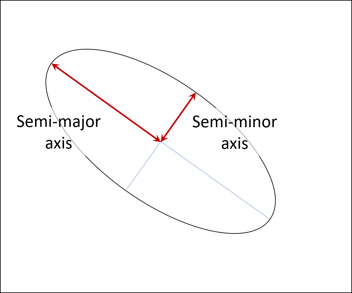
In the previous blog post, Statistics of multi-dimensional data, theory, I introduced a generalization of the standard deviation to three-dimensional data. I called it ellipsification. In this blog post I am going to apply this ellipsification thing to real data to demonstrate the application to statistical process control of color.


I posted this cuz there just aren't enough trolls on the internet
Is the data normal?
In traditional SPC, the assumption is almost always made that the underlying variation is normally distributed. (This assumption is rarely challenged, so we blithely use the hammers that are conveniently in our toolbox -- standard SPC tools -- to drive in screws. But that's another rant.)
The question of normalcy is worth addressing. First off, since I am at least pretending to be a math guy, I should at least pay lip service to stuff that has to do with math. Second, we are venturing into uncharted territory, so it pays to be cautious. Third, we already have a warning that deltaE color difference is not normal. Ok, maybe a bunch of warnings. Mostly from me.
I demonstrate in the next section that my selected data set can be transformed into another data set with components that are uncorrelated, have zero mean and standard deviation of 1.0, and which give every indication of being normal. So, one could us this transform on the color data and apply traditional SPC techniques on the individual components, but you will see that I take this one step further.
I demonstrate in the next section that my selected data set can be transformed into another data set with components that are uncorrelated, have zero mean and standard deviation of 1.0, and which give every indication of being normal. So, one could us this transform on the color data and apply traditional SPC techniques on the individual components, but you will see that I take this one step further.
Original data
I use the solid magenta data from the data set that I describe below in the section below called "Provenance of the data". I picked magenta because it is well known that it has a "hook". In other words, as you increase pigment level or ink film thickness, it changes hue. The thicker the magenta ink, the redder it goes. Note that this can be seen in the far left graph as a tilt to the ellipsoid.
I show three views of the data below. The black ellipses are slices through the middle of the ellipsification in the a*b* plane, the L*a* plane, and the L*b* plane, respectively.

View from above

View from the b* axis

View from the a* axis
Standardized data
Recall for the moment when you were in Stats 201. I know that probably brings up memories of that cute guy or girl that sat in the third row, but that's not what I am talking about. I am talking about standardizing the data to create a Z score. You subtracted the mean and then divided by the standard deviation so that the standardized data set has zero mean, and standard deviation of 1.0.
I will do the same standardization, but generalized to multiple dimensions. One change, though. I need an extra step to rotate the axes of the ellipsoid so that all the axes are aligned with the coordinate axes. The cool thing is that the new scores (call them Z1, Z2, and Z3, if you like) are now all uncorrelated.
Geometrically, the operations are as follows: subtract the mean, rotate the ellipsoid, and then squish or expand the individual axes to make the standard deviations all equal to 1.0. The plot below show three views of the data after standardization. (Don't ask me which axes are L*, a*, and b*, by the way. These are not L*, a*, or b*.)

Standardized version of the L*, a*, and b* variation charts
Not much to look at -- some circular blobs with perhaps a tighter pattern nearer the origin. That's what I would hope to see.
Here are the stats on this data:
| Mean | Stdev | Skew | Kurtosis | |
| Z1 | 0.000 | 1.000 | -0.282 | -0.064 |
| Z2 | 0.000 | 1.000 | 0.291 | 0.163 |
| Z3 | 0.000 | 1.000 | -0.092 | -0.658 |
The mean and standard deviation are exactly 0.000 and 1.000. This is reassuring, but not a surprise. It just means that I did the arithmetic correctly. I designed the technique to do this! Another thing that happened by design is that the correlations between Z1 and Z2, and between Z1 and Z3 are both exactly 0.000. Again, not a surprise. Driving those correlations to zero was the whole point of rotating the ellipsoid, which I don't mind saying was no easy feat.
The skew and kurtosis are more interesting. For an ideal normal distribution, these two values will be zero. Are they close enough to zero? None of these numbers are big enough to raise a red flag. (In the section below entitled "Range for skew and kurtosis", I give some numbers to go by to scale our expectation of skew and kurtosis.)
In the typical doublespeak of a statistician, I can say that there is no evidence that the standardized color variation is not normal. Of course, that's not to say that the standardized color variation actually is normal, but a statement like that would be asking too much from a statistician. Suffice it to say that it walks like normally distributed data and quacks like normally distributed data.


Dr. Bunsen Honeydew lectures on proper statistical grammar
This is an important finding. At least for this one data set, we know that the standardized scores Z1, Z2, and Z3 can be treated independently as normally distributed variables. Or, as we shall see in the next section, we can combine them into one number that has a known distribution.
Can we expect that all color variation data behaves this nicely when it is standardized by ellipsification? Certainly not. If the data is slowly drifting, the standardization might yield something more like a uniform distribution. If the color is bouncing back and forth between two different colors, then we expect the standardized distributions to be bi-modal. But I intend to look at a lot of color to try to see if 3D normal distribution is the norm for processes that are in control.
In the words of every great research paper every written, "clearly more research is called for".
The Zc statistic
I propose a statistic for SPC of color, which I call Zc. This is a generalization of the Z statistic that we all know and love. This new statistic could be applied to any multi-dimensional data that we like, but I am reserving the name to apply to three-dimensional data, in particular, to color data. (The c stands for "color". If you have trouble remembering that, then note that c is the first letter of my middle name.)
Zc is determined by first ellispifying the data set. The data set is then standardized, and then each data point is reduced to a single number (a scalar), as described in the plot below. The red points are a standardization of the data set we have been working with.the data set we have been working with. I have added circles at Zc of 1, 2, 3, 4. Any data points on one of these circles will have a Zc score of the corresponding circle. Points in between will have intermediate values, which are the distance from the origin. Algebraically, Zc is the sum in quadrature of the individual three components, that is to say, the square root of the sum of the squares of the three individual components.

A two-dimensional view of the Z scores
Now that we have standardized our data into three uncorrelated random variables that are (presumably) Gaussian with zero mean and unit standard deviation, we can build on some established statistics. The sum of the squares of our standardized variable will follow a chi-squared distribution, and the square root of the sums of the squares will follow a chi distribution. Note that this quantity is the distance from the data point to the origin.
Chi is the Greek version of our letter X. It is pronounced with the hard K sound, although I have heard neophytes embarrass themselves by pronouncing it with the ch sound. To make things even more confusing, there is a Hebrew letter chai which is pronounced kinda like hi, only with that rasping thing in the back of your throat. Even more confusing is the fact that the Hebrew chai looks a lot like the Greek letter pi, which is the mathematical symbol for all things circular like pie and cups for chai tea. But the Greek letter chi has nothing to do with either chai tea, or its Spoonerism tai chi.
Whew. Glad I got that outa the way.
Why is it important that we can put a name on the distribution? This gives us a yardstick from which to gauge the probability that any given data point belongs to the set of typical data. The table below gives some probabilities for the Zc distribution. Here is an example that will explain the table a bit. The fifth row of the table says that 97% of the data points that represent typical behavior will have Zc scores of less than 3.0. Thus the chance that a given data point will have a Zc score larger than that is 1 in 34.
Levels of significance of Zc
| Zc | P(Zc) | Chance |
| 1.0 | 0.19875 | 1 |
| 1.5 | 0.47783 | 2 |
| 2.0 | 0.73854 | 4 |
| 2.5 | 0.89994 | 10 |
| 3.0 | 0.97071 | 34 |
| 3.5 | 0.99343 | 152 |
| 4.0 | 0.99887 | 882 |
| 4.5 | 0.99985 | 6623 |
| 5.0 | 0.99999 | 66667 |
The graph below is a run time chart of the Zc scores for the 204 data points that we have been dealing with. The largest score is about 3.5. We would be hard pressed at calling this an aberrant point, since the table above says that there is a 1 in 152 chance of such data happening at random. By the way, we had close to 152 data points, so we should expect 1 data point above 3.5. A further test: I count eight data points where the Zc score is above 3.0. Based on the table, I expect about 6.
My conclusion is that there is nothing funky about this data.

Runtime chart for Zc of the solid magenta patches
Where do we draw the line between common cause and special cause variation? In traditional SPC, we use Z > 3 as the test for individual points. Note that for a normal distribution, the probability of Z < 3 is 0.99865, or one chance in 741 of Z < 3.0. This is pretty close to the probability of Zc < 4 for a chi distribution. In other words, if you are using Z > 3 as a threshold for QC with normally distributed data, then you should use Zc > 4 when using my proposed Zc statistic for color data. Four is the new three.
Provenance for this data
In 2006, the SNAP committee (Specifications for Newspaper Advertising Production) took on a large project to come to some consensus about what color you get when you mix specific quantities of CMYK ink on newsprint. A total of 102 newspapers printed a test form on its presses. The test form had 928 color patches. All of the test forms were measured by one very busy spectrophotometer. The data was averaged by patch type, and it became known as CGATS TR 002.
Some of the patches were duplicated on the sheet for quality control. In particular all of the solids were duplicated. Thus, in the blog post, I was dealing with 204 measurements of a magenta solid patch from 102 different newspaper printing presses.
Range for skew and kurtosis
How do we decide when a value of skew or kurtosis is indicative of a non-normal distribution? Skew should be 0.0 for normal variation, but can it be 0.01 and still be normal? Or 0.1? Where is the cutoff?
Consider this: the values for skew and kurtosis that we compute from a data set are just estimates of some metaphysical skew and kurtosis. If we asked all the same printers to submit another data set the following day, we would likely have a somewhat different value of all the statistics. If we had the leisure of collecting a Gillian or a Brilliant or even a vermillion measurements, we would have a more accurate estimate of these statistical measures.
Luckily some math guy figgered out a simple formula that allows us to put a reliability on the estimates of skew and kurtosis that we compute.
Our estimate of skew has a standard deviation of sqrt (6 / N). For N = 204 (as in our case) this works out to 0.171. So, an estimate of skew that is outside of the range from -0.342 to 0.342 is suspect, and outside the range of -0.513 to 0.513 is very suspect.
For kurtosis, the standard deviation of the estimate is sqrt (24/N), which gives us a range of +/- 0.686 for suspicious and +/- 1.029 for very suspicious.